Usage

In the following sections, we look at how to manipulate spectral cubes, including how to convolve and match cubes, and how to make publication ready figures.

Data processing

We have developed a set of functions to help you process your data. This is continuously evolving to include more features to enable individual projects.

Convolve and Match cubes

A common task is to convolve and match the cubes to a common resolution. This is usually required to enable the comparison of different cubes, e.g., to derive abundances or column density ratios. The function regrid_cubes_from_files will take a list of cubes and a template cube. It will convolve the cubes to the smallest beam that is common to all the cubes in the list, and then regrid the cubes to the same resolution as the template cube. The function will also add a suffix to the output files to indicate that they have been convolved and matched. Usually the template file used is the lowest frequency cube, as this is the one that will have the largest beam and pixels.

from prodige_core import data_handler
from glob import glob

# get file list of data cubes
fits_files = glob('HH211*.fits')
# get the template file
template_file = 'HH211_13CO_2-1.fits'
# convolve and match the cubes to the template
data_handler.regrid_cubes_from_files(fits_files,
                                     template_file,
                                     suffix = '_conv_match')

If you only want to convolve the cubes to a common beam, without regridding, it can be done with the function common_beam_files.

from prodige_core import data_handler
from glob import glob

# get file list of data cubes
fits_files = glob('HH211*.fits')
# convolve the cubes to the common beam
data_handler.common_beam_files(fits_files, suffix = '_conv')

Making figures

We developed a set of functions to help you make publication ready figures, which can be used with your own custom made plotting routines. This includes commands with the information of the source names, known outflows directions, primary beam sizes, and other information.

In addition, we have also created a couple of wrapper functions to create publications ready figures with a single command.

Single-pointing Continuum

The function plot_continuum will create a figure with the continuum map of a single pointing observations towards the source, adding the outflow direction, the primary beam size, and the source name. The function will also save the figure in the current working directory with the name of the source and the baseband.

import os
import prodige_core as pcore
# NOEMA data directory
data_directory = os.getcwd() + '/'

# # name of the region
region = 'B5-IRS1'
# continuum baseband
bb = 'lo'
print('>>>>> ' + region + ' continuum of single pointing')
pcore.plot_continuum(region, bb, data_directory, cmap='inferno', mosaic=False,
                    color_nan='0.9', do_marker=True, do_outflow=True,)

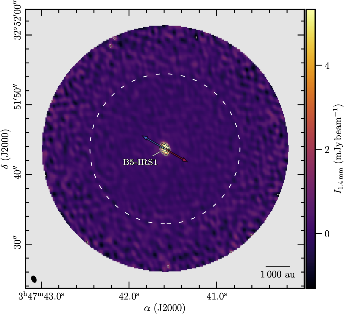
Example of a continuum map of Barnard5-IRS1 with the outflow direction and the primary beam size.

Continuum Mosaic

The function plot_continuum can also handle continuum data from different pointings mosaiced together. the outflow direction, the primary beam size, and the source name. The function will also save the figure in the current working directory with the name of the source and the baseband.

import os
import prodige_core as pcore
# NOEMA data directory
data_directory = os.getcwd() + '/'

# # name of the region
region = 'L1448N'
# continuum baseband
bb = 'li'
print('>>>>> ' + region + ' continuum of Mosaic')
pcore.plot_continuum(region, bb, data_directory, cmap='inferno', mosaic=True,
                    color_nan='0.9', do_marker=True, do_outflow=True,)

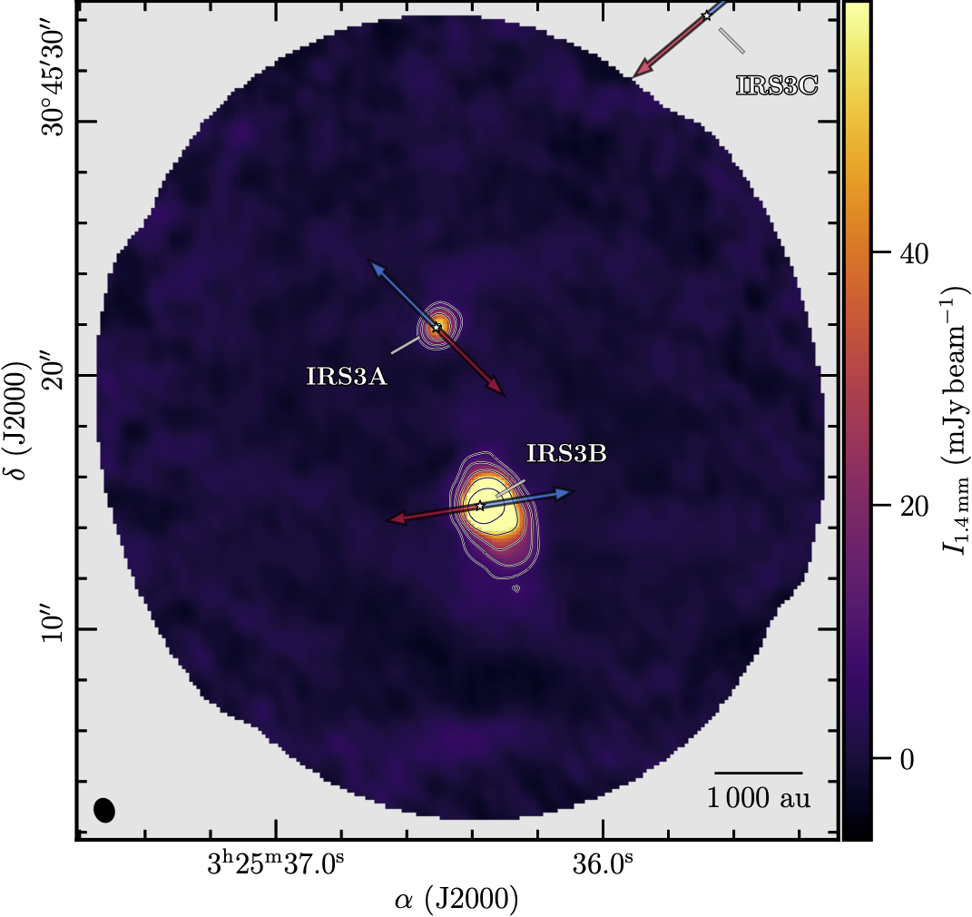
Example of a continuum map of L1448N with the outflow direction.

Line Integrated Intensity Maps

The function plot_line_mom0 will create a figure with the integrated intensity map of a single pointing (or mosaicked) observations towards the source, adding the outflow direction, the primary beam size (for single pointing), and the source name. The function will also save the figure in the current working directory with the name of the source and the baseband.

import os
import prodige_core as pcore
# NOEMA data directory
data_directory = os.getcwd() + '/'

# # name of the region
region = 'HH211'
# linename
linename = 'N2Dp_K'
bb = 'li'
print('>>>>> ' + region + ' Integrated Intensity')
pcore.plot_line_mom0(region, linename, bb, data_directory, mosaic=False,
                    color_nan='0.9', do_marker=True, do_outflow=True,)

Example of a integrated intensity map of HH211 with the outflow direction and the primary beam size.

Centroid Velocity Maps

The function plot_line_vlsr will create a figure with the centroid velocity map of a single pointing (or mosaicked) observations towards the source, adding the outflow direction, the primary beam size (for single pointing), and the source name. The function will also save the figure in the current working directory with the name of the source and the baseband.

import os
import prodige_core as pcore
# NOEMA data directory
data_directory = os.getcwd() + '/'

# # name of the region
region = 'HH211'
# linename
linename = 'N2Dp_K'
bb = 'li'
print('>>>>> ' + region + ' Velocity map')
pcore.plot_line_vlsr(region, linename, data_directory, mosaic=False,
                 color_nan='0.9', do_marker=True, do_outflow=True, do_offsets=True)

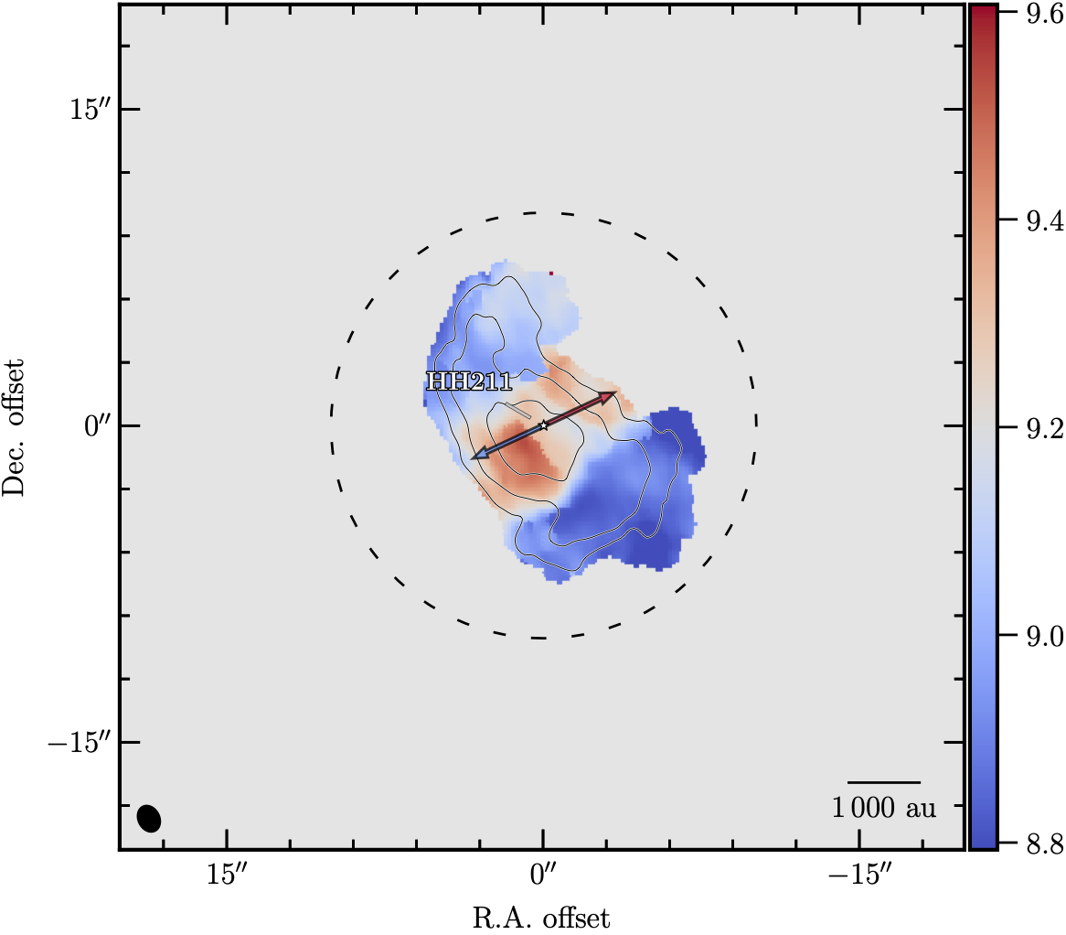
Example of a centroid velocity map of HH211 with the outflow direction and the primary beam size.